Intersect using SpatiaLite

The next step in my geo-experiments journey is to find GPX tracks that pass through an entry polygon and an exit polygon. To start this the GPX needs to be split up into points. For now I used togeojson and will do this in proper Python code later. The resulting "coordinates" list will then be processed via SpatiaLite.

GeoJson

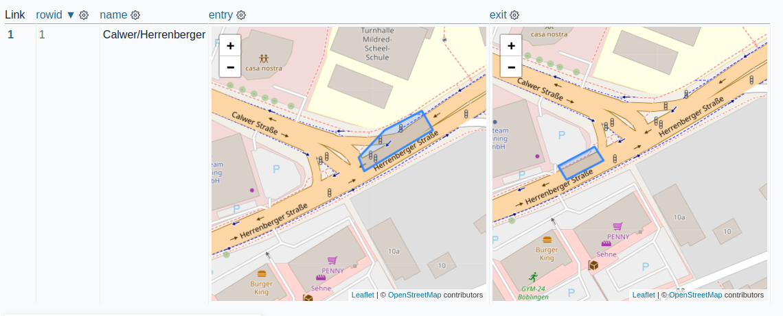
First we need a database entry with one entry polygon and one exit polygon. Using sqlite-utils this could look like this:

DATA=$(cat <<'END_HEREDOC'
{"name": "Calwer/Herrenberger",
 "entry": {"type":"Feature","properties":{"type": "entry"},
   "geometry":{"type":"Polygon",
   "coordinates":[[[9.003386,48.683486],[9.003185,48.68335],[9.003226,48.683275],
     [9.003769,48.683492],[9.003679,48.68359],[9.003386,48.683486]]]}},
 "exit": {"type":"Feature","properties":{"type": "exit"},
   "geometry":{"type":"Polygon",
   "coordinates":[[[9.002798,48.683225],[9.002868,48.683157],[9.002577,48.683058],
     [9.002519,48.683127],[9.002798,48.683225]]]}}}
END_HEREDOC
)
echo $DATA | sqlite-utils insert crossings.db crossings -

The result is a sqlite database with one dataset in the crossings table.

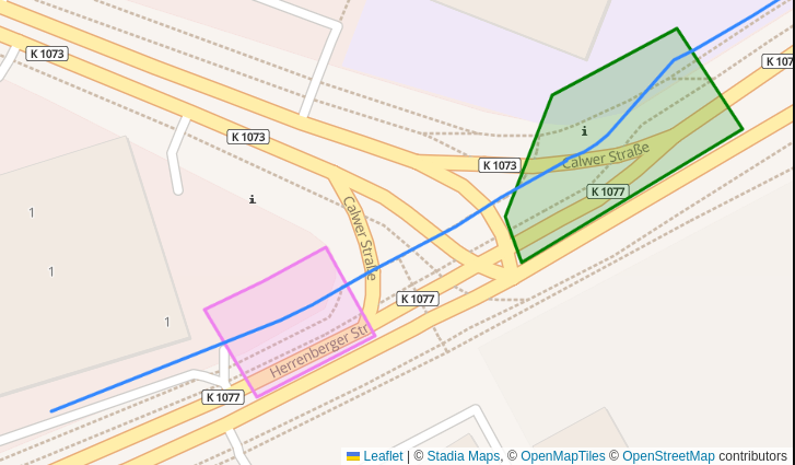
Using Datasette and datasette-leaflet-geojson the imported dataset looks like this:

datasette-preview

One example GPX file cropped to the area that is of interest as GeoJSON:

{"type": "Feature", "geometry": {"type": "LineString", "coordinates": [
[9.004165, 48.683825, 463], [9.004133, 48.683812, 463], [9.004092, 48.683797, 463.2], [9.004047, 48.683779, 463.2],
[9.003999, 48.68376, 463.2], [9.003947, 48.683739, 463.2], [9.003895, 48.683718, 463.4],
[9.003845, 48.683697, 463.4], [9.003795, 48.683676, 463.4], [9.003744, 48.683656, 463.6],
[9.003694, 48.683636, 463.6], [9.003652, 48.683621, 463.6], [9.003619, 48.683609, 463.6],
[9.0036, 48.683603, 463.6], [9.003594, 48.6836, 463.6], [9.003592, 48.683598, 463.6], [9.003592, 48.683598, 463.6],
[9.003592, 48.683598, 463.6], [9.003592, 48.683598, 463.6], [9.003567, 48.683579, 463.6],
[9.003524, 48.683547, 463.6], [9.003495, 48.683526, 463.8], [9.003466, 48.683503, 463.8],
[9.003438, 48.683482, 463.8], [9.003408, 48.683466, 463.8], [9.003378, 48.683455, 463.8],
[9.003354, 48.683447, 463.8], [9.00334, 48.683443, 463.8], [9.003337, 48.683441, 463.8],
[9.003337, 48.683441, 463.8], [9.003337, 48.683441, 463.8], [9.003337, 48.683441, 463.8],
[9.003337, 48.683441, 463.8], [9.003328, 48.683438, 463.8], [9.003304, 48.683428, 463.6],
[9.00327, 48.683415, 463.6], [9.003228, 48.6834, 463.6], [9.003178, 48.683381, 463.4],
[9.003123, 48.683358, 463.2], [9.003064, 48.683334, 463], [9.002998, 48.683309, 463],
[9.002928, 48.683286, 463], [9.002856, 48.683261, 462.8], [9.002785, 48.683234, 462.8],
[9.00271, 48.683207, 462.6], [9.002634, 48.683182, 462.6], [9.002555, 48.68316, 462.6],
[9.002476, 48.683139, 462.4], [9.002398, 48.683118, 462.4], [9.002318, 48.683098, 462.2],
[9.002237, 48.683079, 462.2], [9.002154, 48.683056, 462], [9.002073, 48.683034, 461.8]]}}

Plotted together with the polygons:

track-and-polygons

To create this plot I used leaflet this way:

var example = [
    // entry
    {"type":"Feature","properties":{"type":"entry"},"geometry":{"type":"Polygon","coordinates":[[[9.0033,48.683546],[9.003185,48.68335],[9.003226,48.683275],[9.003769,48.683492],[9.003608,48.683654],[9.0033,48.683546]]]}},
    // exit
    {"type":"Feature","properties":{"type":"exit"},"geometry":{"type":"Polygon","coordinates":[[[9.002745,48.683301],[9.002868,48.683157],[9.002577,48.683058],[9.002447,48.6832],[9.002592,48.683245],[9.002745,48.683301]]]}},
    // track
    {"type": "Feature", "geometry": {"type": "LineString",
            "coordinates": [...<see above>...]}}
        ]

  L.geoJSON(example, {
    style: function(feature) {
        if (feature.properties){
            switch (feature.properties.type) {
                   case 'entry': return {color: "green"}
                   case 'exit':   return {color: "violet"}
            }}}}).addTo(map);

SpatiaLite

But how can we calculate if a track is actually crossing entry and exit in SQL?

First we need libspatialite (for example on ArchLinux):

# https://archlinux.org/packages/extra/x86_64/libspatialite/
pacman -S libspatialite

The next step is to verify via SQL if the track is crossing both polygons. This code needs shapely and sqlite-utils installed.

import json
from shapely.geometry import shape
from sqlite_utils.db import Database

# create a new database
db = Database("crossings_demo.db")

# add the spatialize tables
db.init_spatialite("/usr/lib/mod_spatialite.so")  # path to library file

# table for polygons
table = db["areas"]
table.insert_all([
        {"id": 1, "type": "entry",
            "geojson": {
                "type": "Polygon",
                "coordinates": [
                    [
                        [9.003386, 48.683486], [9.003185, 48.68335], [9.003226, 48.683275],
                        [9.003769, 48.683492], [9.003679, 48.68359], [9.003386, 48.683486],
                    ]]}},
        {"id": 2, "type": "exit",
            "geojson": {
                "type": "Polygon",
                "coordinates": [
                    [
                        [9.002798, 48.683225], [9.002868, 48.683157], [9.002577, 48.683058],
                        [9.002519, 48.683127], [9.002798, 48.683225],
                    ]]}},
    ], pk="id"
)

# add a geometry column
table.add_geometry_column(f"geometry", "POLYGON")

# convert geojson to geometry field
for row in table.rows:
    wkt = shape(json.loads(row["geojson"])).wkt
    db.execute(
        f"update areas set geometry = GeomFromText(?, 4326) where id=?",
        [wkt, row["id"]],
    )

# test if points are in areas
for x, y in (
    (9.003473, 48.683439),  # in entry
    (9.002692, 48.683142),  # in exit
    (9, 48),  # outside of both
):
    r = db.query(
        "select :x, :y, type, WITHIN(MakePoint(:x, :y), areas.geometry) as inside from areas",
        {"x": x, "y": y}
    )
    print(list(r))

# returns
# [{':x': 9.003473, ':y': 48.683439, 'type': 'entry', 'inside': 1},
#  {':x': 9.003473, ':y': 48.683439, 'type': 'exit', 'inside': 0}]
# [{':x': 9.002692, ':y': 48.683142, 'type': 'entry', 'inside': 0},
#  {':x': 9.002692, ':y': 48.683142, 'type': 'exit', 'inside': 1}]
# [{':x': 9, ':y': 48, 'type': 'entry', 'inside': 0}, {':x': 9, ':y': 48, 'type': 'exit', 'inside': 0}]

# query for a track intersection with the entry/exit areas
track = {"type": "LineString", "coordinates": [
  [9.003845, 48.683697], [9.003795, 48.683676], [9.003744, 48.683656],
  [9.003694, 48.683636], [9.003652, 48.683621], [9.003619, 48.683609],
  [9.003592, 48.683598], [9.003592, 48.683598], [9.003567, 48.683579],
  [9.003337, 48.683441], [9.003328, 48.683438], [9.003304, 48.683428],
  [9.00271, 48.683207], [9.002634, 48.683182], [9.002555, 48.68316],
]}

wkt = shape(track).wkt
r = db.query(
  "select type, Intersects(GeomFromText(?), Envelope(areas.geometry)) as crosses from areas",
  [wkt],
)
print(list(r))

# returns
# [{'type': 'entry', 'crosses': 1}, {'type': 'exit', 'crosses': 1}]

Personal todos here:

  • the track Intersects for exit only when using an Envelope around it

  • this could be faster with a SpatialIndex but I couldn't get it to work

  • How is the performance when the track is a lot of points (i.e. 100km gpx file)

Reverse Geo Location

For the drawn polygons I want to add a location label to get an idea where it is without the need of a map.

Nominatim

The standard solution is Nominatim and this would solve my problem easily, i.e. https://nominatim.openstreetmap.org/ui/reverse.html?lat=48.68330&lon=9.00311&zoom=17 (no link to not cause traffic). The query only returns one street and I am actually interested in the crossing of two streets.

The Usage policy of Nominatim could be okish for my idea, but I wanted to explore alternatives.

Stadia Maps

So I looked into what Stadia Maps could do, because I use them for maps already. Using their openapi based reference and a bit of Python code solves my problem (same geo coordinate as above):

import httpx

r = httpx.get(
    "https://api-eu.stadiamaps.com/geocoding/v1/reverse",
    params={
        "point.lat": "48.68330",
        "point.lon": "9.00311",
        "boundary.circle.radius": 1,  # 1 km radius
        "layers": "street",
        "sources": "openstreetmap",
        "api_key": "your-api-key-goes-here",
    },
)

for index, street in enumerate(r.json()["features"]):
    print(
        {
            k: v
            for k, v in street.get("properties").items()
            if k in ["distance", "label", "gid"]
        }
    )
    if index == 4:
        # stop after max 5 streets
        break

This results in:

{'distance': 0.019, 'gid': 'openstreetmap:street:polyline:31083747', 'label': 'Calwer Straße, Böblingen, BW, Germany'}
{'distance': 0.094, 'gid': 'openstreetmap:street:polyline:27779973', 'label': 'Berliner Straße, Böblingen, BW, Germany'}
{'distance': 0.12, 'gid': 'openstreetmap:street:polyline:31083808', 'label': 'Herrenberger Straße, Böblingen, BW, Germany'}
{'distance': 0.167, 'gid': 'openstreetmap:street:polyline:6513917', 'label': 'Karl-Benz-Straße, Böblingen, BW, Germany'}
{'distance': 0.203, 'gid': 'openstreetmap:street:polyline:6508508', 'label': 'Kurze Straße, Böblingen, BW, Germany'}

Which is not perfect, because the crossing is actually between "Calwer Straße" and "Herrenberger Straße". I see where this comes from: The crossing between "Berliner Straße" and "Herrenberger Straße" is not that far away. But overall this is good enough for me, as I only need a hint for a human where the crossing roughly is.

The Stadia Maps reverse api endpoint is in beta and currently free to use, but looking at their pricing table, reverse geo location seems to be not included in the free tier once it is out of beta.

OpenCage

The next possible solution is OpenCage Geocoding API. They have a good demo page too that shows everything I needed. The code to get the nearest street via OpenCage:

r = httpx.get(
    "https://api.opencagedata.com/geocode/v1/json",
    params={
        "q": "48.68330,9.00311",
        "language": "en",
        "key": "your-api-keys-goes-here",
        "pretty": 1,
    },
)

result = r.json()["results"][0]
print(result.get("formatted"))

This results in:

Calwer Straße, 71034 Böblingen, Germany
Like Nominatim this api returns only one street but still a good alternative when Stadia Maps is not free anymore.

Conclusion

I may use both apis (Stadia Maps and OpenCage) in the beginning and wait what happens when the Stadia Maps reverse geolocation feature is out of beta.

There are other alternatives and getlon.lat gives a pretty good overview. For me having three (including Nominatim) solutions seems enough for now.

How to use Pandas in Org Mode

I track my rowing workouts using Strava and a custom rowing counter with my rowing machine. Now a few years later I have nearly 500 rowing workouts and would like to analyse and plot them. Of course I could use a Jupyter Notebook, as always, but this time I wanted to try Org Mode for this.

First step is some setup in the org file.

#+STARTUP: inlineimages

#+BEGIN_SRC emacs-lisp :results none
; use a virtualenv with python created with virtualenv-wrapper
(setq org-babel-python-command "~/.virtualenv/emacs-pandas/bin/python")
; update image after execution of babel
(eval-after-load 'org
  (add-hook 'org-babel-after-execute-hook 'org-redisplay-inline-images))
#+END_SRC

At the beginning of the org file we activate inlineimages. This is important to show the plots later. An alternative to activate is M-x org-toggle-inline-images or C-c C-x C-v. For more information see the org mode manual.

The emacs-lisp babel block solves two problems I had. First my global Python doesn't has Pandas installed, so I created a virtualenv and installed Pandas in there. This virtualenv is referenced here and used as default Python command. This change is global, so be aware all other babel usages of Python will use this virtualenv now.

The last elisp command adds a hook that updates every inline image after a babel block was executed.

Now let us add a bit of data:

#+NAME: rowdata
|         id | moving_time |       date | rows |   rpm |
| 8804906424 |         901 | 2023-03-30 |  388 | 25.84 |
| 8786341302 |         902 | 2023-03-27 |  365 | 24.28 |
| 8775651293 |         902 | 2023-03-25 |  372 | 24.75 |
| 8765797455 |         903 | 2023-03-23 |  382 | 25.38 |
| 6830032281 |         902 | 2022-03-15 |  319 | 21.22 |
| 6819994746 |         903 | 2022-03-13 |  356 | 23.65 |
| 6804568223 |         902 | 2022-03-10 |  294 | 19.56 |
| 6794097174 |         902 | 2022-03-08 |  372 | 24.75 |

The data is on purpose in March in two different years to show grouping by year/month later. moving_time is in seconds and rows is for the whole workout. The rpm value could be calculated here in the table, but I did this when exporting the data. The table got the a name to use in the Python blocks later.

Loading the org table into Pandas works like this:

#+BEGIN_SRC python :var tbl=rowdata :results output
  import pandas as pd

  df = pd.DataFrame(tbl[1:], columns=tbl[0])
  print(df.iloc[:2])
#+END_SRC

Variables from outside the code block are set via :var and the way the result is returned is set via :results. The first column is expected to have the names of the columns.

Running this block (C-c C-c) results in:

#+RESULTS:
:            id  moving_time        date  rows    rpm
: 0  8804906424          901  2023-03-30   388  25.84
: 1  8786341302          902  2023-03-27   365  24.28

How about plots! Org mode can only display files, so every plot has to be saved to disk and the filename has to be returned by the code block.

Example:

#+BEGIN_SRC python :var tbl=rowdata :results file
  import pandas as pd

  filename = "result.png"
  df = pd.DataFrame(tbl[1:], columns=tbl[0])
  p = df.set_index("date").plot(y="rpm", kind="bar")
  # bbox_inches="tight" cuts the image to the correct size
  p.get_figure().savefig(filename, bbox_inches="tight")
  return filename
#+END_SRC

This results in an image like this (inline in the org file):

/images/orgmode-pandas-result.png

Of course the image is now stored in the folder of the org file and can be used/displayed somewhere else.

Finally some more complicated plot: Group the mean of the rpms for every month. To achieve this some pandas magic has to happen.

Example:

#+BEGIN_SRC python :var tbl=rowdata :results file
  import pandas as pd

  filename = "result2.png"
  df = pd.DataFrame(tbl[1:], columns=tbl[0])
  df["date"] = pd.to_datetime(df.date)
  df = df.set_index("date").groupby(pd.Grouper(freq="M")).mean(numeric_only=True)
  # all months in between are set to NaN; remove them
  df = df.dropna()
  # add a year-month column
  df["ym"] = pd.to_datetime(df.index).strftime("%Y-%m")
  p = df.plot.bar(x="ym", y="rpm")
  p.get_figure().savefig(filename, bbox_inches="tight")
  return filename
#+END_SRC

The grouping happens with .groupby(pd.Grouper(freq="M")).mean(). The DatetimeIndex will result in NaNs between the two month we have in the data. To remove them the df.dropna() was added.

The result looks like this (again as inline in the org file):

/images/orgmode-pandas-result2.png

Finally the plot with my actual rowing workouts until today:
/images/orgmode-pandas-rowing-result.png