How to use Pandas in Org Mode
I track my rowing workouts using Strava and a custom rowing counter with my rowing machine. Now a few years later I have nearly 500 rowing workouts and would like to analyse and plot them. Of course I could use a Jupyter Notebook, as always, but this time I wanted to try Org Mode for this.
First step is some setup in the org file.
#+STARTUP: inlineimages

#+BEGIN_SRC emacs-lisp :results none
; use a virtualenv with python created with virtualenv-wrapper
(setq org-babel-python-command "~/.virtualenv/emacs-pandas/bin/python")
; update image after execution of babel
(eval-after-load 'org
  (add-hook 'org-babel-after-execute-hook 'org-redisplay-inline-images))
#+END_SRC
At the beginning of the org file we activate inlineimages.
This is important to show the plots later.
An alternative to activate is M-x org-toggle-inline-images or C-c C-x C-v.
For more information see the org mode manual.
The emacs-lisp babel block solves two problems I had. First my global Python doesn't has Pandas installed, so I created a virtualenv and installed Pandas in there. This virtualenv is referenced here and used as default Python command. This change is global, so be aware all other babel usages of Python will use this virtualenv now.
The last elisp command adds a hook that updates every inline image after a babel block was executed.
Now let us add a bit of data:
#+NAME: rowdata
|         id | moving_time |       date | rows |   rpm |
| 8804906424 |         901 | 2023-03-30 |  388 | 25.84 |
| 8786341302 |         902 | 2023-03-27 |  365 | 24.28 |
| 8775651293 |         902 | 2023-03-25 |  372 | 24.75 |
| 8765797455 |         903 | 2023-03-23 |  382 | 25.38 |
| 6830032281 |         902 | 2022-03-15 |  319 | 21.22 |
| 6819994746 |         903 | 2022-03-13 |  356 | 23.65 |
| 6804568223 |         902 | 2022-03-10 |  294 | 19.56 |
| 6794097174 |         902 | 2022-03-08 |  372 | 24.75 |
The data is on purpose in March in two different years to show grouping by year/month later.
moving_time is in seconds and rows is for the whole workout.
The rpm value could be calculated here in the table, but I did this when exporting the data.
The table got the a name to use in the Python blocks later.
Loading the org table into Pandas works like this:
#+BEGIN_SRC python :var tbl=rowdata :results output
  import pandas as pd

  df = pd.DataFrame(tbl[1:], columns=tbl[0])
  print(df.iloc[:2])
#+END_SRC
Variables from outside the code block are set via :var and the way the result is returned is set via :results.
The first column is expected to have the names of the columns.
Running this block (C-c C-c) results in:
#+RESULTS:
:            id  moving_time        date  rows    rpm
: 0  8804906424          901  2023-03-30   388  25.84
: 1  8786341302          902  2023-03-27   365  24.28
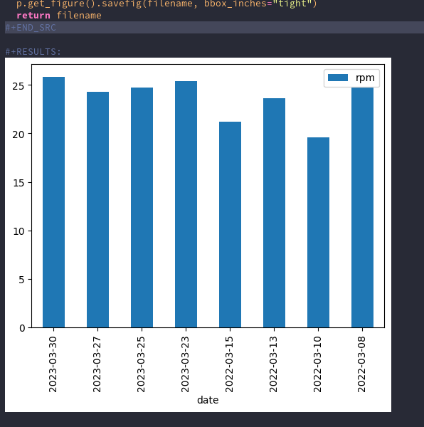
How about plots! Org mode can only display files, so every plot has to be saved to disk and the filename has to be returned by the code block.
Example:
#+BEGIN_SRC python :var tbl=rowdata :results file
  import pandas as pd

  filename = "result.png"
  df = pd.DataFrame(tbl[1:], columns=tbl[0])
  p = df.set_index("date").plot(y="rpm", kind="bar")
  # bbox_inches="tight" cuts the image to the correct size
  p.get_figure().savefig(filename, bbox_inches="tight")
  return filename
#+END_SRC
This results in an image like this (inline in the org file):
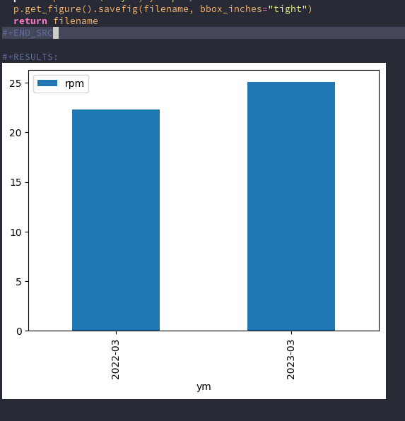
Finally some more complicated plot: Group the mean of the rpms for every month. To achieve this some pandas magic has to happen.
Example:
#+BEGIN_SRC python :var tbl=rowdata :results file
  import pandas as pd

  filename = "result2.png"
  df = pd.DataFrame(tbl[1:], columns=tbl[0])
  df["date"] = pd.to_datetime(df.date)
  df = df.set_index("date").groupby(pd.Grouper(freq="M")).mean(numeric_only=True)
  # all months in between are set to NaN; remove them
  df = df.dropna()
  # add a year-month column
  df["ym"] = pd.to_datetime(df.index).strftime("%Y-%m")
  p = df.plot.bar(x="ym", y="rpm")
  p.get_figure().savefig(filename, bbox_inches="tight")
  return filename
#+END_SRC
The grouping happens with .groupby(pd.Grouper(freq="M")).mean().
The DatetimeIndex will result in NaNs between the two month we have in the data.
To remove them the df.dropna() was added.
The result looks like this (again as inline in the org file):